Tabular

Note

This page describe what is specific to the tabular layout. For more general information creating and using datasets, see Using an existing dataset and Building your own datasets respectively.

Creating

To create a tabular dataset, the layout entry in the recipe’s output section must be set to tabular:

output:
  layout: tabular

Using

To open a tabular dataset, you use the open_dataset function with the start, end, window and frequency parameters.

ds = open_dataset(
    dataset,
    start=1979,
    end=2020,
    window="(-6h,0]",
    frequency="6h",
)

The default values for start and end are the first and last date of the dataset, respectively. Because these value may fall on full round hours, it is recommended to set them explicitly.

Unlike for gridded datasets, the start, end and frequency parameters can have arbitrary values, and are used to define how windows are built and how many samples are in the dataset. Note that start and end can be outside the range of actual dates in the datasets. When requesting windows outside the range of actual dates, empty records will be returned to the user.

The default value for window is (-3h,0] and the default value for frequency is 3h. Windows are relative time intervals that can be open or closed at each end. A round bracket indicates an open end, while a square bracket indicates a closed end. The default units are hours.

Windows can be open or closed at each end:

"[-3,+3]" # Both ends are included
"(-1d,0]" # Start is open, end is closed

Data samples

The dataset is made of samples, which are built by applying the window to a list of reference dates defined by the start, end and frequency parameters.

Reference dates

The references dates of the dataset are defined as all dates between start and end with a step of frequency.

result = []
date = start

while date <= end:
    result.append(date)
    date += frequency

Note

The reference dates are not necessarily the same as the actual dates in the dataset. They are used, together with the window parameter, to define the samples returned when iterating the dataset. See below for more information. Nevertheless, in order to ensure compatibility with gridded datasets, the reference dates are available as the dates attribute of the dataset.

It is not currently possible to combine tabular and gridded datasets within a single call to open_dataset, but when this will be implemented, ds.dates, ds.frequency, len(ds), etc. will all be compatible and comparable between the two layouts.

ds.dates # Returns the list of reference dates defined by start, end and frequency

The number of samples in the dataset is then given by the formula:

number_of_samples = (end - start) // frequency + 1

to get the list of dates, you can access the dates attribute of the dataset:

ds.dates # Returns the list of reference dates defined by start, end and frequency

The length of the dataset is equal to the number of samples:

assert len(ds) == number_of_samples

Single sample

A sample is a 2D numpy array that is returned when indexing the dataset with an integer. The first dimension of the array is the number of observations in the window, and the second dimension is the number of variables. Each sample is constructed by applying the window to the corresponding date. For example, if the date is 2020-01-01 00:00:00 and the window is (-3h,0], then the sample will contain all observations between 2019-12-31 21:00:00 and 2020-01-01 00:00:00, including the latter but not the former.

sample = ds[42]

# A 2D array is returned, the first dimension is the number of observations
# in the 43rd window (samples are 0-indexed).

assert len(sample.shape) == 2

# The second dimension is the variables

assert sample.shape[1] == len(ds.variables)

The whole dataset can also be iterated over using a for loop:

for sample in ds:
    assert len(sample.shape) == 2
    assert sample.shape[1] == len(ds.variables)

is equivalent to:

for i in range(len(ds)):
    sample = ds[i]
    assert len(sample.shape) == 2
    assert sample.shape[1] == len(ds.variables)

Auxiliary information

Becuse tabular data is unstructured, information such as the latidudes, longitudes and dates if the actual data cannot be provided at the dataset level. Instead, it is provided at the sample level. When you access a sample, you can also access the corresponding latitudes, longitudes, dates, etc. This information is returned as attributes of the sample:

Auxiliary information can be accessed as:

sample = ds[42]

number_of_observations_in_window = sample.shape[0]


 # Returns the corresponding latitudes

sample.latitudes

assert len(sample.latitudes) == number_of_observations_in_window

# Returns the corresponding longitudes

sample.longitudes

assert len(sample.longitudes) == number_of_observations_in_window

sample.dates # Returns the corresponding row dates

# Returns the corresponding dates

sample.dates

assert len(sample.dates) == number_of_observations_in_window

# Return the reference date of the window

sample.reference_date

assert sample.reference_date == ds.start_date + 42 * ds.frequency

# Return the timedeltas in seconds relative to the reference_date

sample.timedeltas

assert len(sample.timedeltas) == number_of_observations_in_window

Slices

When slicing the dataset, the same rules apply as for indexing with an integer, but you can recover the samples using the boundaries attribute of the resulting array . The boudaries attribute is a list of slice objects that can be used to access the samples in the result. You also can retrieve the reference dates with the reference_dates attribute of the result.

samples = ds[10:30]

assert len(samples.boundaries) == 20
assert len(samples.reference_dates) == 20

i = 10
for b in samples.boundaries:
      sample = samples[b]
      assert np.array_equal(sample, ds[i])
      i += 1

The latitudes, longitudes, dates, timedeltas, etc. attributes of the resulting array are the concatenation of the corresponding attributes of the samples.

assert np.array_equal(samples.latitudes, np.concatenate([ds[i].latitudes for i in range(10,30)]))

assert np.array_equal(samples.longitudes, np.concatenate([ds[i].longitudes for i in range(10,30)]))

assert np.array_equal(samples.dates, np.concatenate([ds[i].dates for i in range(10,30)]))

Warning

The two codes below are not equivalent:

samples = ds[10:30]
boundaries = samples.boundaries

latitudes = samples.latitudes[boundaries[1]]

and:

samples = ds[10:30]
boundaries = samples.boundaries

latitudes = samples[boundaries[1]].latitudes

Only the first construct will work.

Examples

The following examples show various ways to define the window and the frequency parameters when opening a tabular dataset.

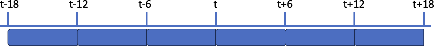
First example, the window width (6h) matches the frequency (6h), so the whole dataset is covered:

ds = open_dataset(
    path,
    start=1979,
    end=2020,
    window="(-6h,0]",
    frequency="6h")

The schema below illustrates the window and frequency parameters in this case:

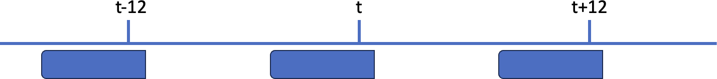
Second example, the window width (6h) is narrower than the frequency (12h), so there are gaps between the windows:

ds = open_dataset(
    path,
    start=1979,
    end=2020,
    window="(-5h,+1h]",
    frequency="12h")

As illustrated in the schema below, there are gaps between the windows:

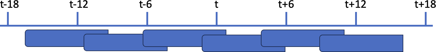
In the third example, the window width (8h) is wider than the frequency (6h), so there are overlaps between the windows:

ds = open_dataset(
    path,
    start=1979,
    end=2020,
    window="(-5h,+3h]",
    frequency="6h")

As illustrated in the schema below, there are overlaps between the windows: